How to draw a free-body diagram in LaTeX using TikZ

Whether you’re writing about physics, vectorial calculus, trigonometry or any other topic that requires a diagram representing the sum of two vectors in a 2D plain, using LaTeX with TikZ makes this process a bit easier with just a few lines of code and a bit of knowledge about trigonometry.

Setting everything up

The first thing we have to do is create a TikZ environment just so we can start seeing immediate results. For a more isolated workflow I’m gonna use a package called standalone which allows the separate PDF compilation of TikZ pictures (cropped to fit the actual size of whatever you draw). In the code you can notice I used the tikz option in the package, which automatically imports TikZ.

\documentclass[tikz]{standalone}

\begin{document}
\begin{tikzpicture}
  % Code goes here
\end{tikzpicture}
\end{document}

You can go ahead and compile it but nothing will be drawn inside the PDF, so let’s start with a simple grid.

Drawing the grid

Any good Cartesian plain needs a grid and 2 axis markers. This time around we won’t be adding measurement lines for simplicity’s sake. The first step is to create the appropriate coordinates: $g_1$ and $g_2$ at points $(-5,-5)$ and $(5,5)$ respectively. These two points represent the start and end points of the grid, from which we can deduce that the size of the grid will be $10cm\times 10cm$.

\coordinate (o)  at (0,0);   % origin
\coordinate (g1) at (-5,-5); % grid bottom left
\coordinate (g2) at (5,5);   % grid upper right

After that, we proceed to draw the axis lines with the \draw command. The necessary setup involves importing the arrows TikZ library to change the default arrow tip and define their line styles (this block goes outside of the document environment):

\usetikzlibrary{arrows}

\tikzset{
  >=stealth', % Change default arrow tip
  grid/.style={step=1cm,gray!30,very thin},
  axis/.style={thick,<->},
}

These styles can also be scoped inside the tikzpicture environment by putting them inside square brackets (options) like this: \begin{tikzpicture}[...].

% Grid rendering (bottom left) -- (upper right).
\draw[grid] (g1) grid (g2);
% Perpendicular X and Y axis.
\draw[axis] (g1 |- o) -- (g2 |- o) node[anchor=east,xshift=15] {x};
\draw[axis] (g1 -| o) -- (g2 -| o) node[anchor=north,yshift=15] {y};

These \draw commands go inside the tikzpicture environment and I performed a clever trick using the |- and -| operators; |- is used to create a coordinate with the $x$ component of the first coordinate and the $y$ component of the second coordinate. The -| operator is used for the same purpose but inverted. In summary, the last 2 commands draw the axis lines.

Once you update your code, compile the document and you’ll be rewarded with:

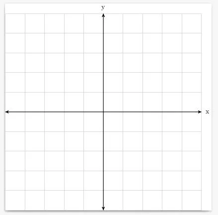
Let’s remember again that the units are given in centimeters.

Vector lines

The next step is to draw the 3 lines corresponding to the sum of two vectors: $F_1$, $F_2$ and $F_R$ (the resulting vector). We could manually input the coordinates for $F_R$ but we can use the calc TikZ library to automatically sum the two vectors and compute its coordinates. But first, we need to define more styles and update the \usetikzlibrary directive:

\usetikzlibrary{arrows,calc}

\tikzset{
  >=stealth', % Change default arrow tip
  grid/.style={step=1cm,gray!30,very thin},
  axis/.style={thick,<->},
  vect/.style={ultra thick,->},
  vnode/.style={midway,font=\scriptsize}
}

We need our vector lines really thick with an arrow tip at the end. As for the node, I chose it to be small (\scriptsize) and placed at the mid point of each line, hence midway. And just like in the previous step, we need to define the actual coordinates of each vector— the origin is the same: $(0,0)$:

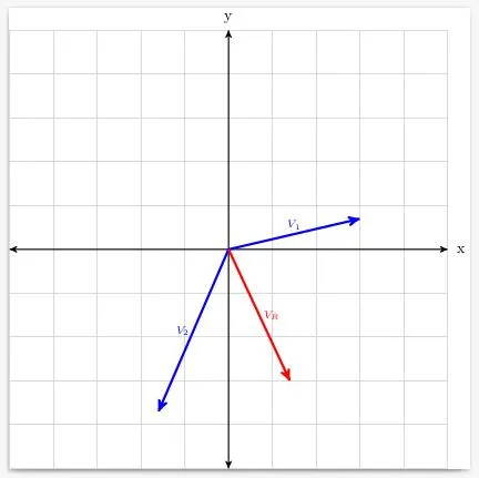
\coordinate (V1) at (3,0.7);
\coordinate (V2) at (-1.6,-3.7);
\coordinate (Vr) at ($(V1) + (V2)$);

Pay absolutely no mind at the random numbers I chose. But do pay attention to the definition of (Vr), this is where the already imported calc TikZ library enters the play, enclosing the expression $(V1) + (V2)$ adds both points and returns the result as a point.

Lastly, we use more \draw commands to actually display these vectors:

\draw[color=blue,vect] (o) -- (V1) node [yshift=6, vnode] {$V_1$};
\draw[color=blue,vect] (o) -- (V2) node [xshift=-7,vnode] {$V_2$};
\draw[color=red, vect] (o) -- (Vr) node [xshift=8, vnode] {$V_R$};

Here’s how it looks after compiling the document:

If when you put your own values for both vector coordinates, the label positions don’t satisfy your needs, you can always edit the xshift and yshift values.

Extra 1 - Angles

Wouldn’t it be nice to have angled semi-circles to represent the apertures of each vector? You can easily add them with a bit of trig knowledge and the math engine of TikZ (you can perform computations with {}). For this task, we’ll need the arc directive inside a \draw command which has 3 parts:

1. Starting angle: We’ll set this at 0 for each arc.
2. Stop angle: This is the real angle and the end of the arc.
3. Radius: As the name suggests, the radius of the semi-circle.

We say that the real angle depends on which quadrant the vector lies in; this means we’ll manually change the code of each arc because not every vector appears in the first quadrant. Here’s the mathematical definition of the relative and real angles for vectors:

In layman’s terms, it means that the real angle is the same as the computed angle if it’s in the first quadrant; you add 180 if it’s in the second or third quadrant; and, you add 360 if it’s in the fourth quadrant.

\draw[color=blue,->] let \p{V} = (V1) in
  (0.75,0) arc (0:{atan(\y{V} / \x{V})}:0.75);
\draw[color=blue,->] let \p{V} = (V2) in
  (0.5,0) arc (0:{atan(\y{V} / \x{V}) + 180}:0.5);
\draw[color=red,->] let \p{R} = (Vr) in              
  (1,0) arc (0:{atan(\y{R} / \x{R}) + 360}:1);

These 3 lines should be grouped with their corresponding vector but for now you can paste them after the vector lines. Compile the document and see the result:

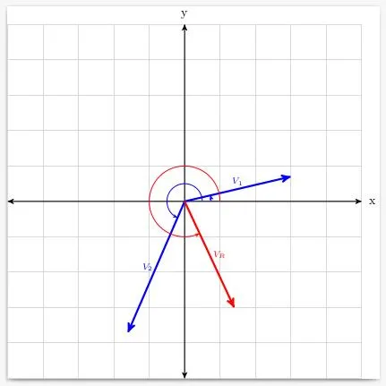
You can play around with the radius of each arc (must match the $x$ component of the coordinate) and the observe how each angle behaves when the corresponding vector is placed in different quadrants.

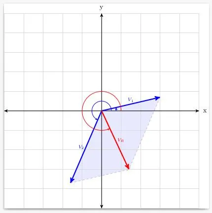
Extra 2 - Parallelogram

Some vector sum diagrams show the parallelogram guide lines. I went above and beyond and not only did I add the guide lines (dashed), but I also added a semi-transparent parallelogram to illustrate how the vector sum works. First we have to edit the style set and add two:

\tikzset{
  >=stealth', % Change default arrow tip
  grid/.style={step=1cm,gray!30,very thin},
  axis/.style={thick,<->},
  vect/.style={ultra thick,->},
  vnode/.style={midway,font=\scriptsize},
  proj/.style={dashed,color=gray!50,->},
  poly/.style={fill=blue!30,opacity=0.3}
}

I chose an opacity of 30% and a light-blue color, but you can change it to what it suits you best. Now all we need is to add two last \draw command and a \fill polygon; all of which must be placed before the vector lines:

% Parallelogram projection lines and polygon.
\draw[proj] (V1) -- +(V2);
\draw[proj] (V2) -- +(V1);
\fill[poly] (o) -- (V1) -- (Vr) -- (V2) -- (o);

The + operator before the second coordinate in each \draw command means that the line will go from the left side coordinate to the point addition of the left side plus the right side, which mathematically means $(a_x + b_x, a_y + b_y)$. Furthermore, the polygon starts from the origin, goes to the tip of $V_1$, then to the tips of $V_R$ and $V_2$, and last, back to the origin. If when you add this code and change the vector coordinates, the polygon becomes skewed in any way, change the path of the polygon until it’s fixed!

The final code

This is the last iteration of the code once I fixed and grouped some things for better readability. You can copy it and paste it, edit the coordinates and most likely, everything will fall into place.

\documentclass[tikz]{standalone}

\usetikzlibrary{arrows,calc}

\tikzset{
  >=stealth', % Change default arrow tip
  grid/.style={step=1cm,gray!30,very thin},
  axis/.style={thick,<->},
  vect/.style={ultra thick,->},
  vnode/.style={midway,font=\scriptsize},
  proj/.style={dashed,color=gray!50,->},
  poly/.style={fill=blue!30,opacity=0.3}
}

\begin{document}
\begin{tikzpicture}
  \coordinate (o)  at (0,0);   % origin
  \coordinate (g1) at (-5,-5); % grid bottom left
  \coordinate (g2) at (5,5);   % grid upper right
  % ---------------------------------------------
  \coordinate (V1) at (3,0.7);
  \coordinate (V2) at (-1.6,-3.7);
  \coordinate (Vr) at ($(V1) + (V2)$);

  % Parallelogram projection lines and polygon.
  \draw[proj] (V1) -- +(V2);
  \draw[proj] (V2) -- +(V1);
  \fill[poly] (o) -- (V1) -- (Vr) -- (V2) -- (o);

  % Grid rendering (bottom left) -- (upper right).
  \draw[grid] (g1) grid (g2);
  % Perpendicular X and Y axis.
  \draw[axis] (g1 |- o) -- (g2 |- o) node[anchor=east,xshift=15] {x};
  \draw[axis] (g1 -| o) -- (g2 -| o) node[anchor=north,yshift=15] {y};

  % Vector angles and lines
  \draw[color=blue,->] let \p{V} = (V1) in
    (0.75,0) arc (0:{atan(\y{V} / \x{V})}:0.75);
  \draw[color=blue,vect] (o) -- (V1) node [yshift=6, vnode] {$V_1$};

  \draw[color=blue,->] let \p{V} = (V2) in
    (0.5,0) arc (0:{atan(\y{V} / \x{V}) + 180}:0.5);
  \draw[color=blue,vect] (o) -- (V2) node [xshift=-7,vnode] {$V_2$};

  \draw[color=red,->] let \p{R} = (Vr) in
    (1,0) arc (0:{atan(\y{R} / \x{R}) + 360}:1);
  \draw[color=red, vect] (o) -- (Vr) node [xshift=8, vnode] {$V_R$};
\end{tikzpicture}
\end{document}